What is run-length ID?
Sometimes during analysis work, you need to group consecutive sequence of values into different “runs”, and calculate metrics for each run. For example:
Given a time series recording some entity’s state, you want to calculate on average, how long does an entity stay in a particular state.
Or a more specific example: Given a series of event data of several users, you want to group the users’ events into sessions with a session cut-off threshold of your choice
This technique is also called sessionization.
Generate run-length ID with R
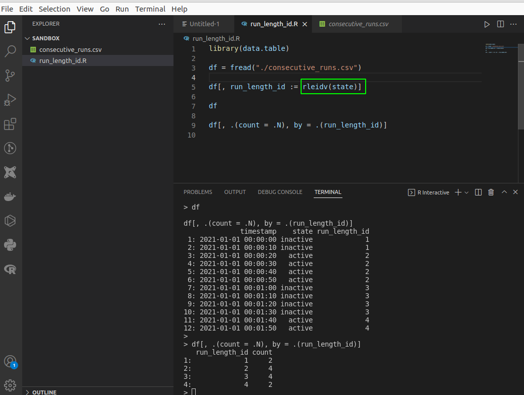
If you are an R user, you may have heard of this kind of analysis. This operation is made trivial with the data.table package, since its rleid/rleidv function can directly generate run-length IDs that are incremented when a new run is commenced.
Since I work most of the time with SQL, sometimes I need to have this kind of behavior in my SQL code. After some experiments, I finally figured out a way to do it. Here’s how:
- First, indexing all the rows in the dataset
- Next, figure out the “points” where the state of your entity changes from one to another by comparing current row and a previous row. ID these “switch points”.
- Use the switch points’ IDs as the ID of the consecutive runs
In this post I will use BigQuery’s Standard SQL to demonstrate how this work, but you can easily implement this in other SQL flavors, as long as your SQL support analytical functions (LEAD, LAG, ROW_NUMBER, FIRST_VALUE, LAST_VALUE…)
Generate run-length ID with SQL
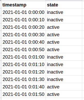
Example: How long does an object stay in a state?
Suppose we have a device with two state (active/inactive) and we periodically record the state of the device at a particular time. We want to calculate how long do they typically stay in a certain state
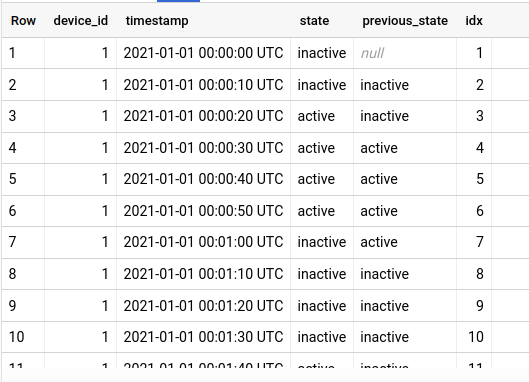
1. Index all rows, and get the previous state
The first step is to create a column containing the previous state, and a “row index” column. We will use the previous_state field to determine the point where the device switch to a new state, and use the idx field to generate the run-length ID.
Since we have multiple devices, we have to partition by device_id when using lag() to make sure we do not get the state of a device into data of another device.
select
  *
  , lag(state, 1) over (partition by device_id order by timestamp) as previous_state
  , row_number() over (order by timestamp) as idx
from test.consecutive_runs
order by device_id, timestamp
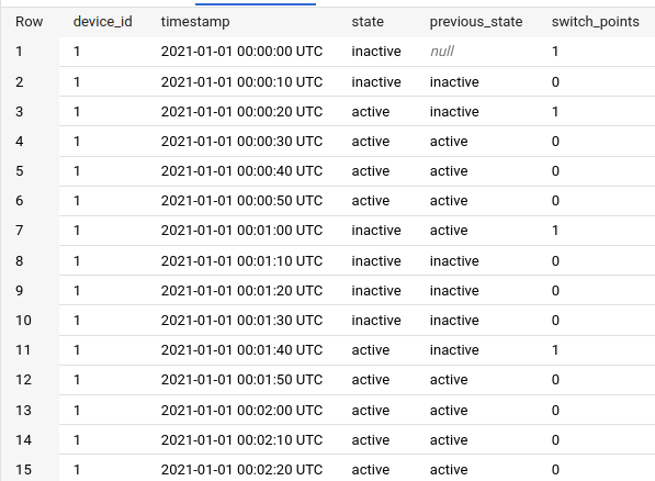
2. Determine the state switching points
Next, we will check for the “switch point”. If an event is a switch point, we will make the idx of that event NULL. This is to prepare for the generation of run-length ID.
with base as (
  select
    *
    , lag(state, 1) over (partition by device_id order by timestamp) as previous_state
    , row_number() over (order by timestamp) as idx
  from test.consecutive_runs
  order by device_id, timestamp
)

select
  *
  , case
      when previous_state is null or state != previous_state
      then idx
    else null end as switch_points
from base
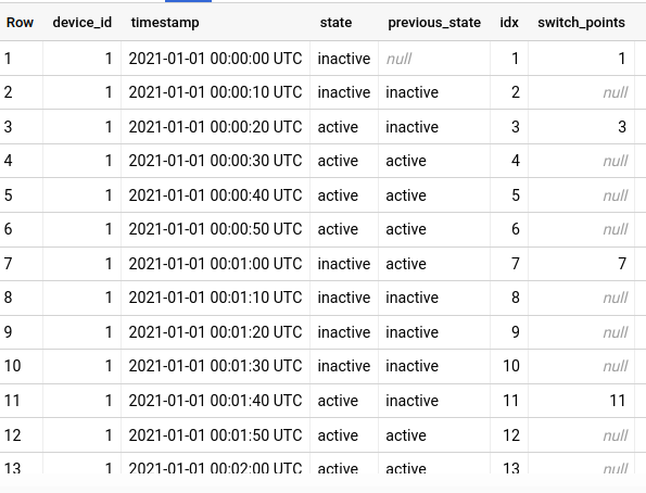
As you can see, row 1 (start of the event series), row 3, row 7 and row 11 are marked as the “switch points”.
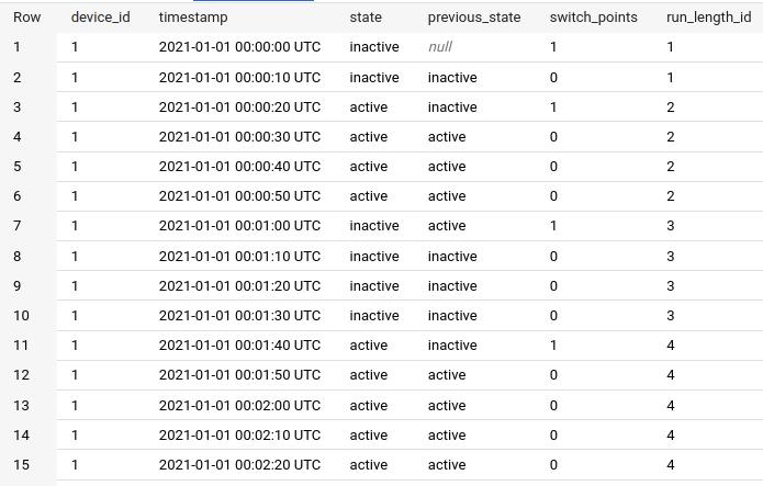
3. Filling in the NULLs
Next we can use the IDs at these switch points to fill the NULL rows below, up to the next switch point. This forward-filling feature can be achieved by BigQuery’s last_value() function:
with base as (
  select
    *
    , lag(state, 1) over (partition by device_id order by timestamp) as previous_state
    , row_number() over (order by timestamp) as idx
  from test.consecutive_runs
  order by device_id, timestamp
)

, switching as (
  select
    *
    , case
        when previous_state is null or state != previous_state
        then idx
    else null end as switch_points
  from base
)

select
  *
  , last_value(switch_points ignore nulls) over (order by timestamp) as run_length_id
from switching
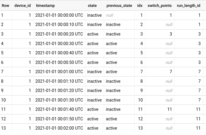
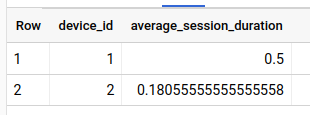
So that’s how we have our run-length IDs. Now we can check on average how long each run lasts:
...

, aggr as (
  select
    device_id
    , run_length_id
    , timestamp_diff(max(timestamp), min(timestamp), second) / 60 as session_duration
  from run_length_table
  group by 1, 2
)

select
  device_id
  , avg(session_duration) as average_session_duration
from aggr
group by 1
4. Another way to generate run-length IDs
In step 2 and 3 above, we made use of NULLs and BigQuery’s last_value() function to generate the IDs. There is another way to generate these IDs using 1, 0 and a moving sum().
Instead of marking “switch points” using idx and set the following row values to NULL, we can mark the switch point using value 1, and set the following rows to 0:
with base as (
  select
    *
    , lag(state, 1) over (partition by device_id order by timestamp) as previous_state
  from test.consecutive_runs
  order by device_id, timestamp
)

select
  *
  , case
      when previous_state is null or state != previous_state
      then 1
    else 0 end as switch_points
from base
Then, use sum(...) over (partition by ...) to perform a running sum of switch points. Whenever the run hits a 1 value, the ID will be increased by one and will stay the same for the next rows (because the next rows are all 0).
with base as (
  select
    *
    , lag(state, 1) over (partition by device_id order by timestamp) as previous_state
  from test.consecutive_runs
  order by device_id, timestamp
)

, switching as (
  select
    *
    , case
        when previous_state is null or state != previous_state
        then 1
      else 0 end as switch_points
  from base
)

select
  *
  , sum(switch_points) over (partition by device_id order by timestamp) as run_length_id
from switching
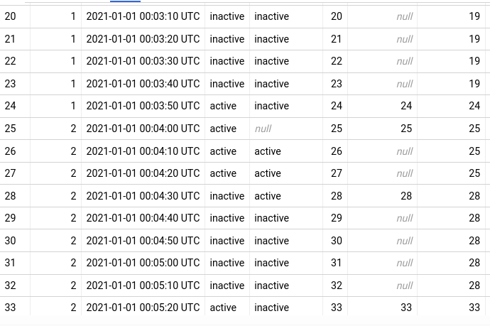
Final result:
Practical use cases for sessionization
This technique can have multiple applications, for example:
- You have records user traffics on your website, but you are not happy with your tracker’s default session grouping. You may want to generate the sessions with your own logic.
- Your have a complex web application, and you have a specific workflow that you want users to go through. You may want to group user’s actions into workflows, and check the ratio of finished over unfinished flows.
Hope that this simple tutorial can give you ideas to solve these kinds of problem.